NGUỒN SÁNG

Tổng quan vê các nguồn sáng liên tục và xung có sẵn
Các loại nguồn sáng liên tục dải rộng1
|
|
Loại nguồn sáng |
Dải bước sóng (nm) |
Công suất quang học dải rộng |
Kích thước điểm hội tụ |
Thông tin khác |
|---|---|---|---|---|---|
LSH-D
|
Deuterium |
185 tới 400 nm |
milliwatts |
22 mm |
|
PowerArc™
|
Xe, Hg hoặc HgXe Arc |
180 tới 1,100 nm |
7 tới 20 watts |
2 tới 10 mm |
|
KiloArc™
|
Xe, Hg hoặc HgXe Arc |
180 tới 1,100 nm |
100 watts |
2 tới 10 mm |
|
LSH-T
|
Tungsten Halogen |
350 tới 2,400 nm |
1 tới 2 watts |
10 tới 12 mm |
|
LSH-GB
|
Glow Bar |
1 tới 15 µm |
milliwatts |
10 tới 18 mm |
|
1 Lưu ý rằng nguồn sáng liên tục có thể "xung" từ 0 - 500 Hz với bộ tạo xung quang học
Các loại nguồn sáng điều hướng liên tục2
|
|
Loại nguồn sáng |
Dải bước sóng (nm) |
Công suất điều hướng quang h |
Thông tin khác |
|---|---|---|---|---|
LSH-D + Monochromator |
Deuterium plus monochromator3 |
180 tới 300 nm |
~ 0.1 tới 1 milliwatts |
|
Tunable PowerArc™
|
Xe arc lamp plus monochromator |
180 tới 1,100 nm |
~ 1 tới 10 milliwatts |
|
Tunable KiloArc™
|
Xe arc lamp plus monochromator |
180 tới 1,100 nm |
~ 10 tới 100 milliwatts |
|
LSH-T + Monochromator |
Tungsten Halogen plus monochromator |
350 tới 2,400 nm |
~ 0.2 tới 2 milliwatts |
|

2 Lưu ý rằng các nguồn sáng liên tục có thể "xung" trong khoảng từ 0 tới 500 Hz với bộ tạo xung quang học
3 Các nguồn sáng điều hướng dựa trên đèn xenon độc đáo của HORIBA hoạt động tốt hơn nguồn sáng điều hướng dựa trên deuterium, ngay cả trong dải UV
|
|
Loại nguồn sáng |
Thời gian xung |
Tốc độ lặp lại |
Dải bước sóng (nm) |
Độ rộng dải phổ |
Thông tin khác |
|---|---|---|---|---|---|---|
SpectraLED
|
LED |
100 ns tới ms |
0.1 tới 10 KHz |
265 tới 1,275 |
10-20 nm |
|
NanoLED
|
LED or Laser Diode |
1.2 tới 1.6 ns |
Lên tới 1 MHz |
250 tới 740 |
10-20 nm |
|
DeltaDiode
|
LED hoặc Laser Diode |
45 tới 350 ps |
Lên tới 100 MHz |
375 tới 1,310 |
7 tới 15 nm |
|
OL-4300 |
Nitrogen Gas Laser |
1.5 ns |
0 tới 20 Hz |
337.1 |
0.1 nm |
|
OL-4300/401
|
Nitrogen Pumped Dye Laser |
1.5 ns |
0 tới 20 Hz |
337.1, 350 tới 990 |
1 tới 3 nm |
|
OL-4300/402 |
Nitrogen Pumped Dye Laser |
1.5 ns |
0 tới20 Hz |
337.1, 350 tới 990 |
0.04 nm |
|
OL-4300/402/403
|
Frequency Doubled, Nitrogen Pumped Dye Laser |
1.5 ns |
0 tới 20 Hz |
235 tới 990 |
0.04 nm |
|


Nhà sản xuất: HORIBA Scientific
Các nguồn sáng của HORIBA được sử dụng kết hợp với các linh kiện quang điện tử và phần mềm tương thích để xây dựng giải pháp quang phổ tùy ý khách hàng.

HORIBA cung cấp các loại nguồn sáng năng lượng cao sử dụng để mô phỏng năng lượng mặt trời và quang điện. Nguồn sáng đèn hồ quang xenon của HORIBA được sử dụng rộng rãi để mô phỏng mặt trời trên toàn thế giới. PowerArc và KiloArc là 2 loại nguồn sáng lý tưởng cho ngành năng lượng mặt trời bởi các nguồn sáng này cung cấp nhiều công suất quang học hơn và ít tốn kém hơn với thiết kế nhỏ gọn và tiện dụng. HORIBA không cung cấp các bộ mô phỏng mặt trời hoặc bộ lọc khối khí (AM), tuy nhiên, nếu khách hàng không cần bộ mô phỏng mặt trời được chứng nhận bởi nhà máy mà đơn giản chỉ tìm kiếm nguồn đèn xenon tốt nhất trên thị trường, chúng tôi có thể mời quý khách tham khảo nguốn sáng PowerArc và KiloArc. Chúng tôi cũng cung cấp các thấu kính chuẩn trực và bộ khuếch đại quang học để hỗ trợ truyền ánh sáng.
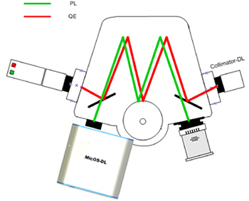
Ngoài các nguồn sáng năng lượng mặt trời, HORIBA Scientific còn cung cấp nguồn sáng điều hướng sử dụng để phân tích hiệu suất lượng tử ngoài (EQE) hoặc hiệu suất chuyển đổi dòng photon thành điện (IPCE) cho nhiều thiết bị năng lượng mặt trời khác nhau.
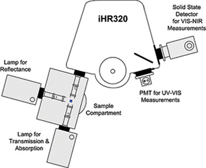
Hấp thụ, Truyền qua và Phản xạ là những công nghệ được sử dụng rộng rãi để xác định tính chất của vật liệu. HORIBA cung cấp nhiều nguồn sáng dải rộng và điều hướng để thực hiện các phép đo này từ UV tới NIR.
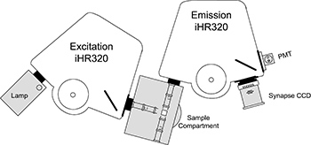
Với các nguồn sáng của HORIBA Scientific, khách hàng có thể thiết kế máy quang phổ huỳnh quang sử dụng các nguồn kích thích cũng như các buồng mẫu, máy quang phổ và detector từ các dải sản phẩm và phụ kiện của HORIBA. Hệ thống điều khiển hoàn chỉnh có sẵn trong phần mềm Syner JY. Chúng tôi cũng bán riêng các loại nguồn sáng để khách hàng có thể nâng cáp và hiện đại hóa các máy huỳnh quang cũ.
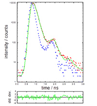
- Sample: Erythrosin B in water (µM)
HORIBA Scientific cung cấp các nguồn sáng LED xung và Diode laser chuyên dụng để nghiên cứu thời gian sống huỳnh quang và phát quang. Những nguồn sáng này được cung cấp dưới dạng hệ thống độc lập hoặc là một bộ phận của các thiết bị huỳnh quang thời gian sống đếm photon đơn tương quan thời gian (TCSPC). Tuy nhiên, nếu bạn đã có các linh kiện phát hiện TCSPC hoặc muốn xây dựng một hệ thống TCSPC tùy ý, bạn có thể kết hợp các công nghệ nguồn sáng tiên tiến này vào hệ thống của bạn.
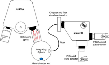
HORIBA Scientific cung cấp các nguồn sáng điều hướng theo ý khách hàng có thể được sử dụng để hiệu chuẩn detector. Chúng tôi có thể thiết kế nguồn sáng hiệu chuẩn hoàn chỉnh đáp ứng các yêu cầu về detector bao gồm các phụ kiện xử lý mẫu và/hoặc các quả cầu tích hợp để chiếu sáng tại những khu vực nhất quán.
Các nguồn sáng xung nano giây có thể được sử dụng để hiệu chuẩn detector thời gian.
Learn more about light sources:
While lenses are used in the examples that follow, front surface concave mirrors coated for the spectral region of choice are preferred. A coating such as aluminium is highly reflective from 170 nm to the near IR whereas crown and flint glasses start losing transmission efficiency rapidly below 400 nm. "Achromatic Doublets" are routinely cemented with UV absorbing resins and their antireflective coatings often discriminate against the UV below 425 nm (this is due to the fact that such lenses are often used in cameras where photographic film may be very UV sensitive).
If lenses must be used in the blue to UV, then choose uncoated quartz singlets or air spaced doublets.

Figure 22. Typical Monochromator System
AS aperture stop
L1 lens 1
M1 mirror 1
M2 mirror 2
G1 grating 1
p object distance from lens L1
q image distance from lens L1
F focal length of lens L1
d the clear aperture of the lens (L1 in diagram)
The above diagram shows a typical monochromator system with one fixed exit slit and one detector, however, all that follows is equally applicable to a spectrograph.
Thin lens equation:
 (3-16)
Magnification (m):
 (2-14)
For simplicity the diameter of an optic or that of its aperture stop (AS) (assuming it is very close to the optic itself) is used to determine the f/value. In which case Equations (2-4) and (2-5) simplify to:
f/valuein = p/d object f/value (6-1)
f/valueout = q/d image f/value (6-2)
- HeNe laser
- Lenses, mirrors, and other optical components as required for optimization (see Section 3)
- Three pinhole apertures of fixed height above the table
- Precision positioning supports for above
- Optical bench, rail, or jig plate
Assemble the above components so that the laser beam acts as the optical axis which passes first through two pinhole apertures, followed by the monochromator, and finally through the third pinhole aperture.
The external optics and source will eventually be placed on the optical axis defined by the pinhole apertures and laser beam. Position the pinhole apertures so that the lenses, etc. may be added without disturbing them.
Note: Reverse illumination may sometimes be preferred where the laser passes first through the exit slit and proceeds through all the optics until it illuminates the light source itself.
Alignment of the components is an iterative process. The goal is for the laser beam to pass through each slit center and to strike the center of each optical element. The following steps achieve this:
- If a monochromator has a sine drive, then set the monochromator to zero order.
- Aim the laser beam through the center of the entrance slit.
- Center the beam on the first optic.
- Center the beam on the next optic, and so on until it passes through the center of the exit slit.
- If the laser does not strike the center of the optic following the grating, then rotate the grating until it does. Many spectrometers are not accurately calibrated at zero order, therefore, some offset is to be expected.
If a light source such as a sample or a calibration lamp is to be focused into the entrance slit of a spectrometer, then:
Ensure that the first active optic is homogeneously illuminated (plane mirrors are passive).
Place a white screen between the entrance slit and the first active optic (in a CZ monochromator, the collimating mirror and in an aberrationcorrected concave grating, the grating itself).
Check for "images", if there is a uniform homogeneously illuminated area, all is well. If not, adjust the entrance optics until there is.
The majority of commercial spectrometers operate between f/3 and f/15, but the diagrams that follow use drawings consistent with f/3 and all the calculations assume f/6.
In the examples which follow, the lens (L1) used is a single thin lens of 100 mm focal length (for an object at infinity) and 60 mm in diameter.
The f/valueout of the entrance optics must be equal to the f/valuein of the monochromator.
If necessary, an aperture stop should be used to adjust the diameter of the entrance optics.
Remember when calculating the diameter of aperture stops, to slightly underfill the spectrometer optics to prevent stray reflections inside the spectrometer housing.
Example 1 (Figure 23)
The emitting source is smaller in width than the width of the entrance slit for a required bandpass.

Figure 23. Small Source Case
1. Calculate the entrance slit width for appropriate bandpass (Equation 3-9). For this example, let the slitwidth be 0.25 mm.
Example Object: a fiber of 0.05 mm core diameter and NA of 0.25.
Object emits light at f/2 (NA = 0.25). Spectrometer = f/6.
2. Projected image size of fiber that would be accommodated by the system (given by entrance slit width) = 0.25 mm.
Calculate magnification to fill entrance slit.
m = image size/object size = 0.25/0.05 = 5.0.
Therefore, q/p = 5, q = 5p.
Substituting into the lens Equation 3-16 gives p = 120 mm, and q = 600 mm.
To calculate d, light must be collected at f/2 and be projected at f/6 to perfectly fill the grating.
Therefore, p/d = 2, d = 120/2 = 60 mm.
Therefore, aperture stop = full diameter of L1.
Projection f/value = 600/60 = 10.
In other words, the grating of the monochromator, even though receiving light collected at f/2, is underfilled by the projected cone at f/10. All the light that could have been collected has been collected and no further improvement is possible.
Example 2
If, however, the fiber emitted light at f/1, light collection could be further improved by using a lens in the same configuration, but 120 mm in diameter. This would, however, produce an output f/value of
600/120 = f/5
Because this exceeds the f/6 of the spectrometer, maximum system light collection would be produced by a lens with diameter
d = q/(f/value) = 600/6 = 100 mm
thereby matching the light collection etendue to the limiting etendue of the spectrometer.
The collection f/value is, therefore,
f/valuein = p/d = 120/100 = 1.2
Since etendue is proportional to the square of the (f/value)-1, about 70% of the available emitted light would be collected at f/1.2 (see Section 3).
If the user had simply placed the fiber at the entrance slit with no entrance optics, only 3% of the available light would have been collected (light in this case was collected at the spectrometer's f/6 rather than the f/1.2 with etendue matching entrance optics).

Figure 24. Extended Souce Case
The object width is equal to or greater than the entrance slit width (see Figure 24).
The f/valueout of the entrance optics must be equal to the f/valuein of the monochromator. The object distance should be equal to the image distance (absolute magnification, m, equals 1).
Aperture stops should be used to match etendue of the entrance optics to the monochromator. Because the object is larger than the slit width, it is the monochromator etendue that will limit light collection.
In this case, image 1:1 at unit magnification.
1. Taking lens L1
So for F = 100 mm, p = 200 mm, q = 200 mm (2F).
2. f/value of the monochromator = q/d = p/d = 6.
Then
d = q/(f/value) = 200/6 = 33.3
Therefore, aperture stop = 33.33 mm to fill the diffraction grating perfectly.
In this case the f/value of the source is numerically larger than that of the spectrometer. This is often seen with a telescope which may project at f/30 but is to be monitored by a spectrometer at f/6. In this case etendue matching is achieved by the demagnification of the source (see Figure 25).

Figure 25. Demagnified Source Case
1. Calculate the entrance slitwidth for the appropriate bandpass(Equation (2-21)). Take, for example, 1.0 mm = final image size = entrance slit width.
2. Image projected by telescope = 5 mm and forms the object for the spectrometer.
m = 1/5 = 0.2,
then from Equation (3-16). Taking lens L1 with F = 100 mm (given),
p = 600 mm, q = 120 mm.
Calculate d knowing the monochromator f/value = 6.
q/d = 6, d = 120/6 = 20 mm.
The aperture stop will be 20 mm diameter.
Light is gathered at either the aperture of the projected image or 600/20 = f/30, whichever is numerically greater.
The concepts given in this section have not included the use of field lenses. Extended sources often require each pupil in the train to be imaged onto the next pupil downstream to prevent light loss due to overfilling the optics, vignetting (see Section 2.8).
- Used when entrance slit height is large and the light source is extended.
- A field lens images one pupil onto another. In Figure 26, AS is imaged onto G1.
Field lenses ensure that for an extended source and finite slit height, all light reaches the grating without vignetting. In Figures 26 and 27 the height of the slit is in the plane of the paper.

Figure 26. Example of Field Lens Imaging One Pupil onto Another

Figure 27. Example of Illumination System with Field Lens
When entrance optics are absent, it is possible for the entrance slit to project an image of just about everything before the slit into the spectrometer. This may include the lamp, the sample, rims of lenses, even distant windows. Section 3 describes how to correctly illuminate a spectrometer for highest throughput. Following this procedure will eliminate the pinhole camera effect.
Multiple imaging may severely degrade exit image quality and throughput. On the other hand, the pinhole camera effect is very useful in the VUV when refractive lenses are not available and mirrors would be inefficient.
Aperture and field stops may be used to reduce or even eliminate structure in a light source, and block the unwanted portions of the light (e.g., the cladding around an optical fiber). In this capacity, aperture stops are called spatial filters (see Figure 28).
The light source image is focused onto the plane of the spatial filter, which then becomes the light source for the system.

Figure 28. Spatial Filter Case